Yorg the image organizer
Yorg is a photo management tool that includes some image
analysis modules to assist the user organizing her data. This document
is a short user manual of the software. The less useful functions are
not described.
1. Before
Download the software from http://lear.inrialpes.fr/src/yorg/
Install the software according to the instructions in the README file.
Launch the program from its main directory with
source setvars.bash
python organizer_gui.py
2. Windows
There are two main windows.
2.1 Database window
This window is visible at startup.
To add images to the collection (= database), use the Database > Add images... menu
and select a directory (not a set of images).

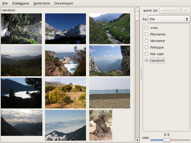
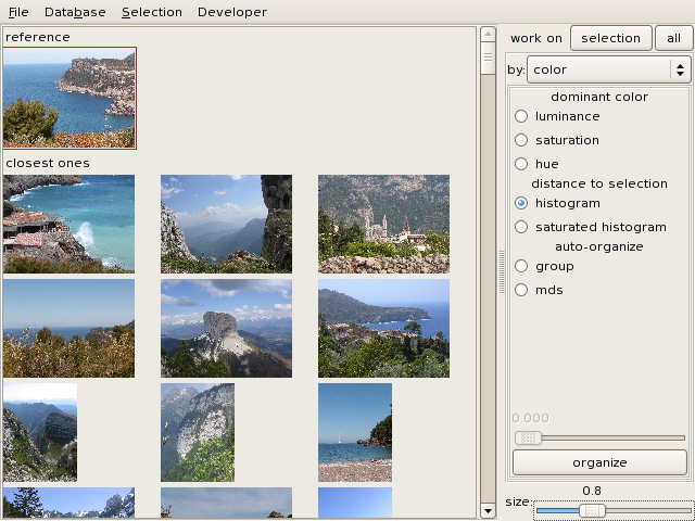
The left pane shows the images of the current database as thumbnails.
The pane at the right shows different organization options. The size slider resizes the thumbnails.
Images can be selected by clicking or drawing a rectangle around them.
The displayed images can be restricted to a subset of the database with
the work on selection button (work on all switches back to the
whole collection).
The file menu has the usual
items. The image collections are stored in a directory rather than a
file. By convention, the extension of the directory name is .iorg. The collection's images
themselves are not stored, so if they are moved somewhere else, they
will be lost
when the collection is re-opened.
2.2 Selection window
Open this window via Selection >
Selection window.

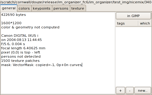
It displays information about the selected image(s). There are
several tabs showing different types of information.
Click on in GIMP to open the
image(s) in the GIMP.
3. Information about images & organization modes
Information can be extracted from each image in the collection. A
series of analysis modules perform more or less complicated analysis
taks on an image. The results, image attributes,
are shown in the selection window.
In the database window, the images can be organized according to one or
several
attributes. The attribute used is selected in the by: dropdown menu on the right,
which shows the appropriate pane.
The attributes are computed when needed, but this often introduces
tedious delays in the GUI. Therefore, you can
explicitly request an analysis of the whole collection via the Database > Analyze... menu items
and go for a cup of tea while the computer works.
3.1 File information
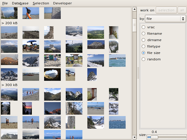
This is the most basic organization type, based only on the image file
attributes (name, size, extension, etc.). Clicking on a radio menu item
immediately orders the collection according to the selected attribute.
vrac means "without a particular order" (but it at least
reflects the order in which the images were added).
Here, images are ordered by file size:

3.2 Exif information
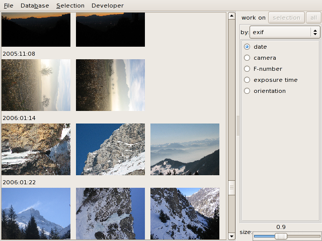
JPEG images generated by most digital cameras contain EXIF
meta-information.
For example, you can order the images by the date they were shot:

3.3 Tags
You can manually annotate images with tags (=keywords).
3.3.1 Defining and assigning tags
Open the selection window to define or add tags to images.
Create a new tag with the new...
button. Enter its name (without spaces) in the dialog box.
The defined tags appear in the first column of a table (the tag list).
The which column indicates
how many among the selected images have this tag.
You can assign tags to the currently selected image(s) in two ways:
- by double-clicking on the appropriate tag in the tag list
- by selecting one or several tags (shift-click) in the list and
use the + (plus) button.
Tags can be un-assigned from the selected images with the - button.
3.3.2 Organizing with tags
You can use tacgs to select the images to display in the database window.
To display images having a given tag, double-click on that tag in the
database window's tag list.
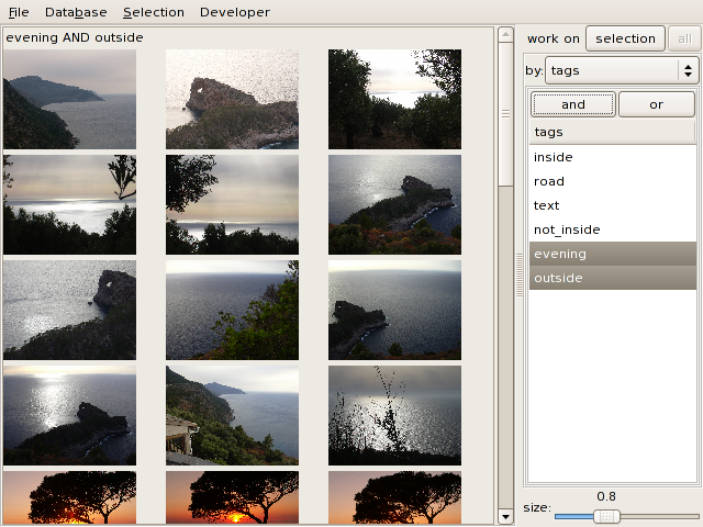
Select several tags (shift-click) in the list and click on the and or or button to compute a boolean
combination of tags. Here, the images having both the evening and outside tags are displayed:

3.3.3 Tips
If you need complex boolean combinations of tags, use re-tagging. For
example:
- to compute (evening AND
outside)
OR road, select all the images of the output of evening AND outside as shown above,
select the output and assign the selection a tag like evening_and_outside. That tag can
then be re-used in an OR expression.
- to compute NOT inside,
display the inside images,
select them and click on Selection
> invert. Then tag all selected images (none of which is
displayed in the database window) with not_inside.
Use tags to keep selections or search results from the other modules.
3.4 Color
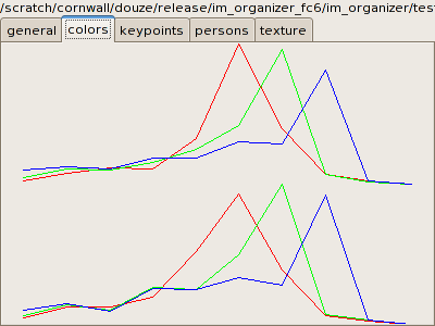
Yorg extracts global color histograms from the images. They are
full 3D histograms with 10*10*10 bins. A reduced version of the
histogram, as separate R, G and B histograms can be displayed in the color
tab of the selection window:

In the database window, the images can be ordered by luminance, hue or
saturation of their average color.
When a reference image is selected, you may order the rest of the
collection by increasing color distance to this image:

The color distance used is the Earth Mover Distance.
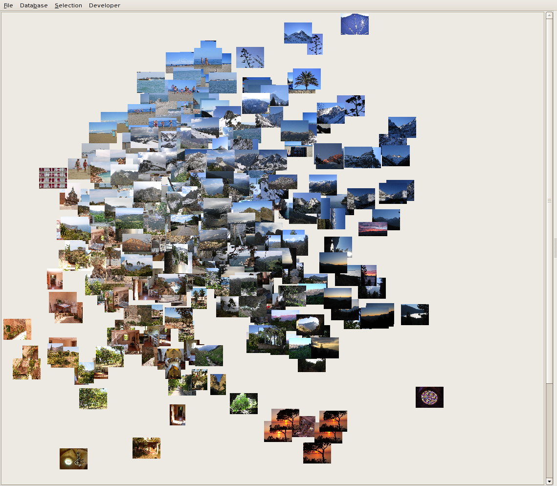
You can also arrange the images in a diagram that attempts to group
close images (in terms of color distance). All pairwise
distances must be computed (slow!). This is done with a
Multi Dimensional Scaling algorithm (MDS):

Since there is no spatial information in the color histograms and
because of the very relative way humans perceive colors, the ordering
based only on a dominant color often seems non-intuitive.
Representations based on distances between color histograms are more
useful.
This part is inspired and based on EMD code by Yossi Rubner (Y. Rubner,
L. Guibas, C. Tomasi, The Earth Mover's Distance, Multi-Dimensional
Scaling and Color-Based Image Retrieval, ARPA Image Understanding
Workshop, 1997).
3.5 Geometry
The images are analyzed to extract keypoints. The keypoints can be
matched to find correspondances between images.
3.5.1 Viewing correspondances
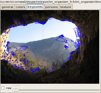
The keypoints tab of the
selection window displays the keypoints of an image.

The blue parallelograms indicate a region used to compute the
keypoint's signature.
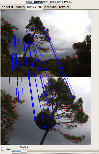
When two images are selected, the tab displays the matched keypoints:

By default, matches are filtered to show only the ones that are
geometrically coherent (e.g. there must be an affine 2D transform that
maps the set of points on one image onto the set on the second).
Ticking the raw option shows
correspondances without this geometric check.
3.5.2 Image distances
The number of matching keypoints can be interpreted as a "geometrical
distance" between images. The smaller this distance, the more likely it
is that the images show the same scene.
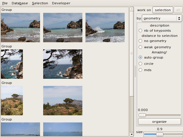
You can group similar images together in the database window according
to this distance:

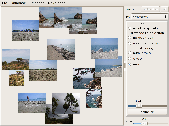
You can also use the distance to make an MDS diagram:

3.6 Person detection
Yorg can detect persons on the images. The detector works best on
upright and entirely visible persons.
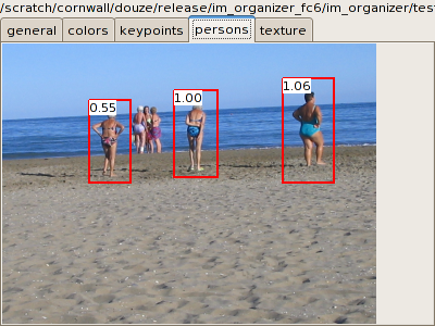
You can see detected persons in the persons
tab of the selection window:

The number in the corner of the detected bounding box is a confidence
value.
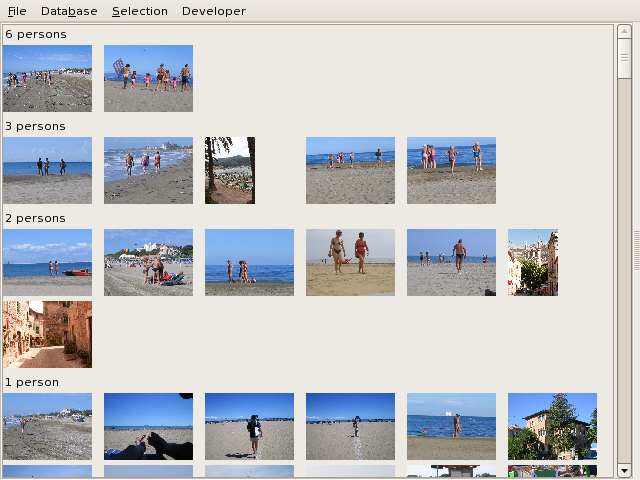
In the collection window, you can order the images by the number of
detected persons:

3.7 Texture
3.7.1 Recognizing textures
Yorg is able to recognize textured zones in the images. Given a kind of
texture to recognize, it extracts patches from each image and evaluates
whether the patch contains that texture.
You can choose the texture of interest in the texture bar of the collection
window.
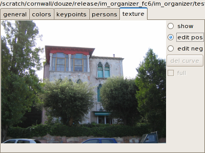
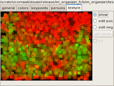
The patches defined in an image are displayed in the texture tab of the selection window
(a foliage texture in this case):


Each patch has a shade between red and green, green indicating that the
current texture is recognized in the patch.
3.7.2 Classification based on textures
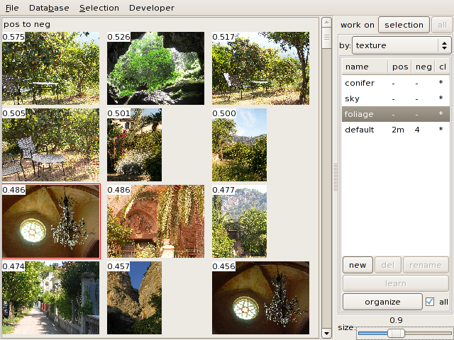
You can order the collection of images by the amout of the texture they
contain. For example, this is the collection ordered by the amount of
foliage:

The figures (between 0 and 1) in the corners of the images indicate
their amount of texture. By default, for speed reasons, clicking on organize only handles a subset of
the database (30 images). Checking the all box orders the whole database.
3.7.3 User-defined texture classifiers
You can define new texture classifiers by indicating positive and
negative image regions. Let's assume that you want to recognize a sea
texture:
- Click on new in the
texture area of the database window. This adds a line in the list, that
can be renamed to "sea".
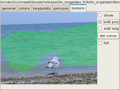
- Select a few sea images. In the texture tab of the selection
window, click on edit pos and
draw a region freehand. It appears in green:

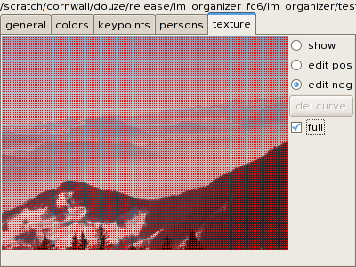
- Negative regions must also be defined. For example, select an
image that does not contain the texture and make a completely negative
region on it (with edit neg
and full):

- Click on learn in the
texture pane to train the classifier.
In the texture list, the second and third columns indicate how many
regions are defined. (1+2m = 1 full image + 2 images with drawn
regions). The fourth column has a "*" if a classifier was trained.
After training, the texture classifier can be used like the predefined
ones.
3.7.4 Tips
Do not expect too much from this image analysis: it recognizes only
simple textures. Selecting cars or faces will not learn an object
detector.
Very often, there are more negative training examples than positive
ones. This explains why the image patches are mostly red. This is not a
problem however, since only relative amounts of texure coverage are
used.
The learning time and storage is grows with the number of example
patches and thus images. To avoid too big an overhead, do not use more
than 4 to 6 training images.
3.8 Refinement
The attributes extracted by the previous modules can be combined to
quickly find images from a few examples. To do this, go to the refine pane in the database window.
Select a few images you like and click on positive. Select a few irrelevant
images and click on negative.
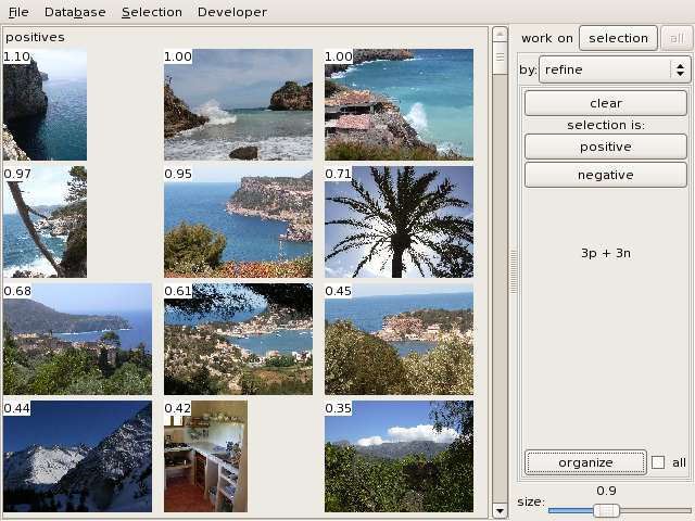
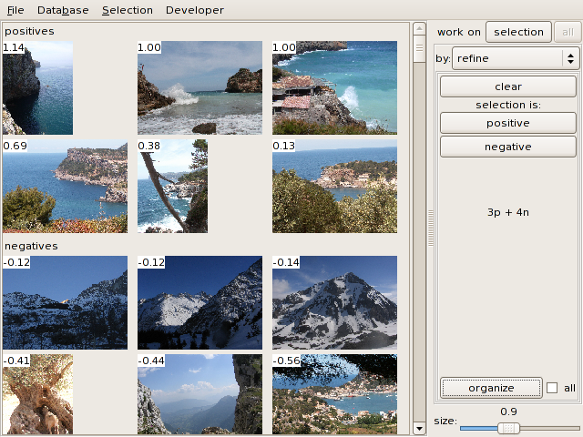
The pane shows something like 3p + 4n, which means 3 positive images
and 4 negative ones.
Click on organize. Here
again, only a subset of images is organized by default (unless all is checked). Yorg allows asks
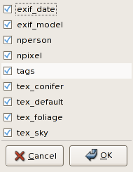
what attributes of the images should be used:

Attribute names should be self-explanatory: exif_* refers to exif
information, nperson and npixel to the number of persons and pixels,
and tex_* are the texture classifier results. You can uncheck the
attributes you think are not relevant, or too slow to compute, etc.
This is an example result where we search for rocks next to the sea
(the figures are confidence values):

The 6th image is wrong, so select it and click on negative and organize. The second classification
is much faster.

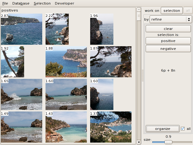
After a few refinement iterations, you can classify the whole set:

If you want to cancel the whole process, click on clear.
This classifier uses an SVM and has many integer or boolean attributes.
Therefore, adding similar images to the positive or negative sets may
not change the ordering at all (the support vectors are the same).
Refrain from adding only negative images, the positive and negative
sets should remain balanced.
4. Miscelaneous
A lot of information is written to the console. If there is a Python
exception (which should not happen, of course), it is caught by the
GUI, which does not exit: it just prints a stacktrace to the console.
If you want, you can send me
this information as a bug report. Of course, C and C++ errors crash the
application.
4.1 Tag import/export
Tags can also be imported and exported with Database > load tags and Database > save tags. They are
stored as a serialized (= "pickled") Python data structure:
stored=(tag_list,tag_dict)
tag_list= all defined tags, as a list of strings
tag_dict= dictionary that maps an image filename to a list of tags
associated with the image.
4.2 Built-in debugger
The menu item Developer > debugger
opens a python debugger command line which allows to examine data, set
breakpoints, etc.
