Estimating the Fundamental Matrix

  

Figure 5.2: An example of automatic epipolar geometry computation

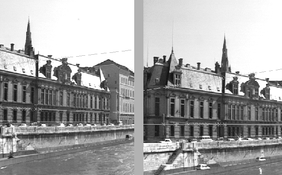
To obtain the epipolar geometry, we need to estimate F. This can be done using some initial point correspondences between the images. Equation (5.3) shows that each matching pair of points between the two images provides a single linear constraint on F. This allows F to be estimated linearly (up to the usual arbitrary scale factor) from 8 independent correspondences. However, F as defined has only seven degrees of freedom: 2 from C (the epipole position) and 5 from A. Algebraically, F has 9 linear coefficients modulo one overall scale factor, but the rank 2 condition implies the additional constraint $\det{(F)}=0$. Hence, F can actually be computed from only 7 matches in general position plus the rank constraint. However, since the latter is a cubic there will generally be three possible solutions in this case.

Figure 5.2 shows what can be done with a good automatic epipolar geometry algorithm. However, for good results, some care is needed. The discussion below is inspired by a paper of R. Hartley [8].

Assume that we have already found some matches $m \leftrightarrow m'$between the images. Each correspondence provides a linear constraint on the coefficients of F: $\;\;m'^{t}Fm=0$. Expanding, we get:

xx'f₁₁ + xy'f₁₂ + xf₁₃ + yx'f₂₁ + yy'f₂₂ + yf₂₃ + x'f₃₁ + y'f₃₂ + f₃₃ = 0

where the coordinates of m and m' are respectively (x, y, 1)^tand (x',y',1)^t. Combining the equations obtained for each match gives a linear system that can be written A f = 0, where f is a vector containing the 9 coefficients of F, and each row of A is built from the coordinates m and m' of a single match. Since Fis defined only up to an overall scale factor, we can restrict the solution for f to have norm 1. We usually have more than the minimum number (8) of points, but these are perturbed by noise so we will look for a least squares solution:

$$\min_{\Vert f \Vert =1} \Vert A f \Vert^2$$

As $\Vert Af\Vert^{2} =~ f^{t} A^{t}Af$, this amounts to finding the eigenvector associated with the smallest eigenvalue of the $9\times 9$symmetric, positive semidefinite normal matrix A^tA. There are standard numerical techniques for this [20]. However, this formulation does not enforce the rank constraint, so a second step must be added to the computation to project the solution F onto the rank 2 subspace. This can be done by taking the Singular Value Decomposition of F and setting the smallest singular value to zero. Basically, SVD decomposes F in the form

F = Q D R

where D is diagonal, and Q and R are orthogonal. Setting the smallest diagonal element of D to 0 and reconstituting gives the desired result.

The above method is standard, but if applied naïvely it is quite unstable. A typical image coordinate in a $512\times 512$ image might be $\sim 200$. Some of the entries in a typical row of A are $xx'\sim 200^2$, others are $x\sim 200$, and the last entry is $1\sim 1$, so there is a variation in size of $\sim 200^2$ among the entries of A, and hence of $200^4\sim 2\cdot10^9$ among the entries of A^tA. This means that numerically, A^tA is extremely ill-conditioned: the solution contains an implicit least squares trade off, but it is nothing like the trade off we would actually like for maximum stability.

A simple solution to this is to normalize the pixel coordinates from [0,512] to [-1,1] before proceeding. This provides a well-balanced matrix A and much more stable and accurate results for F. In a practical implementation, a considerable effort must also be spent on rejecting false correspondences in the input data [27].

In summary, the procedure for estimating the epipolar geometry is:
-- Extract points from the images
-- Find an initial set of point correspondences (typically using correlation)
-- Use the above fundamental matrix estimation algorithm
-- Embed everything in a robust estimation framework resistant to outliers (e.g using Least Median Squares).

For a detailed discussion of alternatives to this scheme, see [12].